$200 vs $200k: Generating Item Features With an LLM Instead of Hand Tagging
A controlled two-tower recommender experiment on MovieLens 32M — and what it means for a team setting up recommendations with no tagging budget.
A hand-curated tag genome and LLM-extracted features are the same idea, one generation apart. Both turn cheap signals into a dense, per-item content matrix. The first took fifteen years of community data. The second needs nothing but an item’s public web text — synopsis, cast, plot, scraped and run through an LLM — and it built the whole corpus in a day.
TL;DR
You’re building a recommender. You’ve got user interactions and each item’s text. What you don’t have: a tagging team, or much of the curated metadata that makes a dataset like MovieLens unusual. So the question is simple. Is a per-item content vector worth building, and can you build it on the cheap?
MovieLens’s gold-standard tag genome took fifteen years of community data to assemble. The cheap version — scrape each item’s text, pull features out with an LLM — covered all ~9,375 movies in a day for about $200 in API calls. And in that bare-bones setting it beats a pure-CF floor and edges the genome on the genome’s own axes: MRR 0.1155 (LLM) / 0.1148 (genome) / 0.1121 (floor). As good as the option you can’t afford. And it’s the one you can actually ship.
See it live — a pixar animation query in the deployed app.
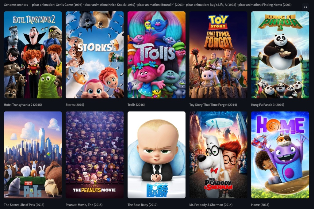
The deployed recommender these features power. A user’s taste vector comes entirely from movie content — the curated genome tags plus the web-scraped, LLM-extracted features this post compares — with no user-ID embedding.
1. The content-feature problem, and the realistic setting
A two-tower recommender turns each item into an embedding. Collaborative signal — who watched what — does most of the work for popular items. But it dries up right where you need help most: the long tail, and brand-new items nobody has touched yet. That’s the job of a content vector. It’s a dense, per-item descriptor of what the item is, no matter who’s interacted with it. The only question is where it comes from.
| Option 1 — the genome | Option 2 — LLM extraction | |
|---|---|---|
| What it is | The gold standard: a dense matrix of rel(movie, tag) ∈ [0,1], every cell populated — 1,128 tags × 16,376 movies (≈18M scores) in this project’s MovieLens 32M data (9,734 movies in GroupLens’s original 2014 release). | Score the item against a fixed tag taxonomy straight from its own public text — the content vector falls out of the item’s description, with no pre-built artifact required. |
| Catalog coverage | Only the well-tagged head: those 16,376 movies are just ~19% of MovieLens 32M’s 87,585 titles. Dense within its coverage, but it simply does not exist for the sparser ~71k (a structural limit we return to in §8). | Any title with public text — no coverage ceiling. |
| How it’s built | Not mass human labeling (the part most people get wrong), but a 50,203-judgment survey of 676 volunteers (1–5 scale; a fraction of a percent of the matrix; plus an 85-user pilot), the rest filled by machine learning (a glmer regression, MAE 0.211) over features mined from a large, pre-existing body of free-form community tags — 186,000 users, 17M ratings, 246,000 tag applications since 1997 — plus crawled IMDb reviews. | Scrape the item’s public text (TMDB synopsis, cast, Wikipedia plot) and ask an LLM to score it, with structured (JSON-schema) output (pipeline in §3). |
The setting that frames the whole experiment. A team standing up recommendations for a fresh catalog starts with way less than MovieLens hands you:
- Doesn’t have: the genome’s inputs — years of community tagging, crawled reviews, a relevance survey. And it’s missing most of the other curated metadata MovieLens ships with: clean, professionally-assigned genre labels on every title, plus 306 high-frequency user tags distilled from a huge crowd-tagging effort.
- Reliably has: interaction logs and an item’s public text. And those interactions are usually implicit — a click, a watch, a purchase — not the 1–5 explicit ratings MovieLens hands out.
So the real question isn’t “genome vs LLM in a metadata-rich model.” It’s this: in the bare setting a real team actually starts from, does a content vector help at all — and is the LLM’s good enough to be the one you build?
2. Why it’s a fair fight
I wanted to compare content sources and nothing else, so everything else stays fixed. Same two-tower architecture. Same training recipe. Same evaluation. Only the content slot changes:
- A — MovieLens genome tags: the 1,128-dim genome scores fill the content tower.
- B — LLM feature tags: 132 LLM-extracted dims fill it instead.
- C — no content tags: the content slot is gone. This is the floor — what the model scores on its history pool and whatever else is around.
(Throughout, A / B / C are the three content arms — genome / LLM / no-content. The main experiment runs them in a base model; §6 re-runs them in a metadata-rich one.)
In that base model — the three arms written C′ / A′ / B′ (floor / genome / LLM) — only the content tower differs:
| Arm | User tower | Item tower | Params |
|---|---|---|---|
| C′ — no content | 1×sum_pool_id(32) = 32 | movieId(32) = 32 | 383,840 |
| A′ — + genome | 1×sum_pool_id(32) + genome_ctx(32) = 64 | genome(32) + movieId(32) = 64 | 472,480 |
| B′ — + LLM | 1×sum_pool_id(32) + llm_ctx(32) = 64 | llm(32) + movieId(32) = 64 | 408,736 |
Same single history pool, same shared item-ID embedding, same projection head, same data, same loss, same 160k-step schedule. The content tower is the only structural difference — and, per the params, genome’s is the largest of the three.
Nothing in the setup favors the LLM. Two deliberate handicaps push the other way, and the one real asymmetry is neutral at best:
- The LLM is boxed into genome’s own taxonomy. Its 132-dim schema is derived from genome’s top-discriminability tags, not hand-invented, so both spaces measure the same axes. (Otherwise “LLM ≈ genome” means nothing.) That makes the question as sharp as it gets: can LLM extraction match the curated genome on its home turf, tag for tag? The LLM gets no credit for patterns it could pull from text but genome never tagged.
- It isn’t even allowed to draft its own. This handles the obvious objection — “a greenfield team has no taxonomy to extract against.” It doesn’t need one. An LLM can draft the taxonomy too, clustering recurring themes across thousands of plots. I deliberately didn’t, to keep the fight fair. The genome dependency is a rule I imposed on this experiment, not a requirement of the method. So if anything, the result understates what an unconstrained LLM pipeline could do.
- The one real asymmetry — compression — is neutral at best. Genome feeds 1,128 raw dims into the content tower, the LLM only 132, but both squeeze down to the same 32. So genome takes the harder compression. That’s routine and usually helps — you want the model finding signal, not memorizing cells. If it tips anything, it doesn’t tip toward the LLM.
Where this sits. LLM-manufactured item features aren’t new. There’s an active 2023–25 line of work — KAR, ONCE/GENRE, LLMRec, RLMRec, with KAR reporting a production A/B gain at Huawei. What’s new here is the comparison. Instead of a weak or absent baseline, this pits the LLM against the gold-standard human-curated genome, on the same axes, with a no-content floor (C) to measure the lift — in the bare setting most teams actually deploy from.
3. The cheap pipeline
Here’s the number you’ll care about first: the entire corpus was scraped and feature-extracted in a single day. One engineer, no annotation team. Each item gets scored on its own, so the work is parallel — hundreds of model-hours of extraction fan out across concurrent calls and wrap up inside a day. Now set that against the genome’s binding input: fifteen years of accrued community data, or the weeks-to-months of fresh tagging it’d take to bootstrap even a rough stand-in.
The pipeline. For each of the ~9,375 corpus movies (9,366 scraped successfully):
- Scrape — TMDB first: overview, tagline, genres, top-billed cast, director, writers, keywords. Then Wikipedia plot and factual prestige indicators on top (Oscar wins/noms, Criterion status, box-office scale).
- Extract — six grouped structured-output calls (themes, tone, setting/era, provenance/structure, factual reception/prestige, visual medium), ~20–30 dimensions each, every call locked to a JSON schema. The grouping is deliberate. A single 130-dim prompt hits “lost in the middle” and defaults the late dimensions to 0.5. Six focused calls don’t.
A few honest design calls are baked in:
- Structured output is non-negotiable. Free-form silently corrupts the tensor.
- The visual and prestige groups are factual-only. Animation, black-and-white, Oscar-winner — yes. “Visually stunning” hallucinated from a synopsis — no.
- Reception/prestige is its own group so it can be ablated on its own.
- Extractor: Claude Sonnet via Claude Code.
What comes out — three fingerprints. Nothing below is hand-picked or tuned. These are the raw six-call outputs for three very different films, side by side, top scores per group (each 0–1):
| Feature Group | 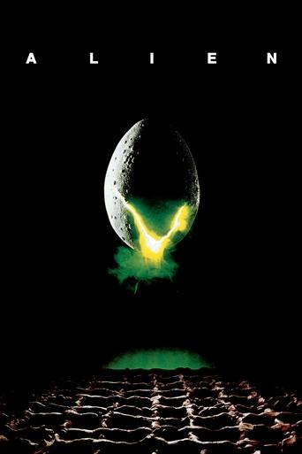 Alien (1979) |
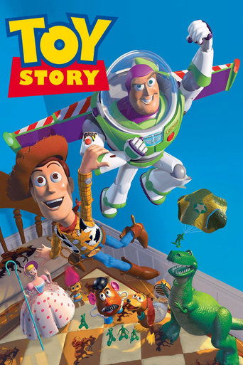 Toy Story (1995) |
 Before Sunrise (1995) |
|---|---|---|---|
| Themes & plot | survival 1.0, betrayal 0.7, mortality 0.7 |
friendship 0.9, family 0.7 |
romance 1.0, relationships 0.9, existentialism 0.6 |
| Tone & mood | tense 1.0, dark 0.9, atmospheric 0.9, creepy 0.9 |
feel_good 0.9, comedic 0.8, emotional 0.6 |
intimate 0.9, reflective 0.8, emotional 0.7 |
| Setting, era & sub-genre | space 1.0, aliens 1.0, monster 0.9, future 0.7 |
small_town 0.4 |
— |
| Provenance & structure | franchise 0.8, twist_ending 0.7 |
franchise 0.9 |
character_study 0.6, independent_film 0.5 |
| Factual reception & prestige | oscar_technical 1.0, classic 0.9, cult_classic 0.6 |
oscar_nominated 0.9, classic 0.8 |
— |
| Visual medium | cgi_heavy 0.3 |
animated 1.0, computer_animation 1.0 |
— |
Every score reads right, and each fingerprint scales to its film. Alien fills every group (cgi_heavy only 0.3 — practical effects, not CG). Toy Story pegs animated / computer_animation at 1.0 and runs feel_good / comedic where Alien runs tense / dark. And Before Sunrise — two strangers talking through one night — comes back honestly spare: a perfect romance 1.0 and an intimate, reflective tone, with almost nothing for the genre, visual-medium, or prestige groups to grab onto. It even half-catches Europe at france 0.2, just under the bar. The extractor reports what’s in the text and nothing more. Same six calls, three very different films, from public text alone.
4. Does it work? — the universal setting
The base model is what any team actually has on day one. Just the two universal signals, with none of MovieLens’s curated privileges:
- Lacks: the curated genre one-hot, the 306 user tags, release year — metadata most catalogs don’t ship with. It also drops the rating-derived history pooling (separate “liked,” “disliked,” and rating-weighted pools), which needs the explicit 1–5 ratings that implicit-feedback systems — clicks, watches — just don’t have.
- Has: a single implicit history pool — the sum of the ID embeddings of the items a user touched, no ratings — plus the content slot under test. That’s it. This is the setting 90%+ of real recommenders live in: “here’s what this user touched, here’s what each item is.”
Call the three arms in this base model C′ / A′ / B′ (floor / genome / LLM). The eval is the same throughout: a held-out rollback protocol — for each validation user, context = history so far, target = next watch — over all 19,134 validation users, n = 382,138 examples. (Random Hit@250 baseline = 2.7%, so these models are doing real work.) A smaller Phase 1 corpus of the 4,461 most-rated movies gives an independent replication.
Primary result — full corpus (n = 382,138):
| Metric | C′ — pure CF floor | A′ — + genome | B′ — + LLM |
|---|---|---|---|
| Hit@5 | 0.1500 | 0.1538 | 0.1555 |
| Hit@10 | 0.2178 | 0.2229 | 0.2236 |
| Hit@50 | 0.4560 | 0.4644 | 0.4647 |
| NDCG@10 | 0.1259 | 0.1290 | 0.1297 |
| MRR | 0.1121 | 0.1148 | 0.1155 |
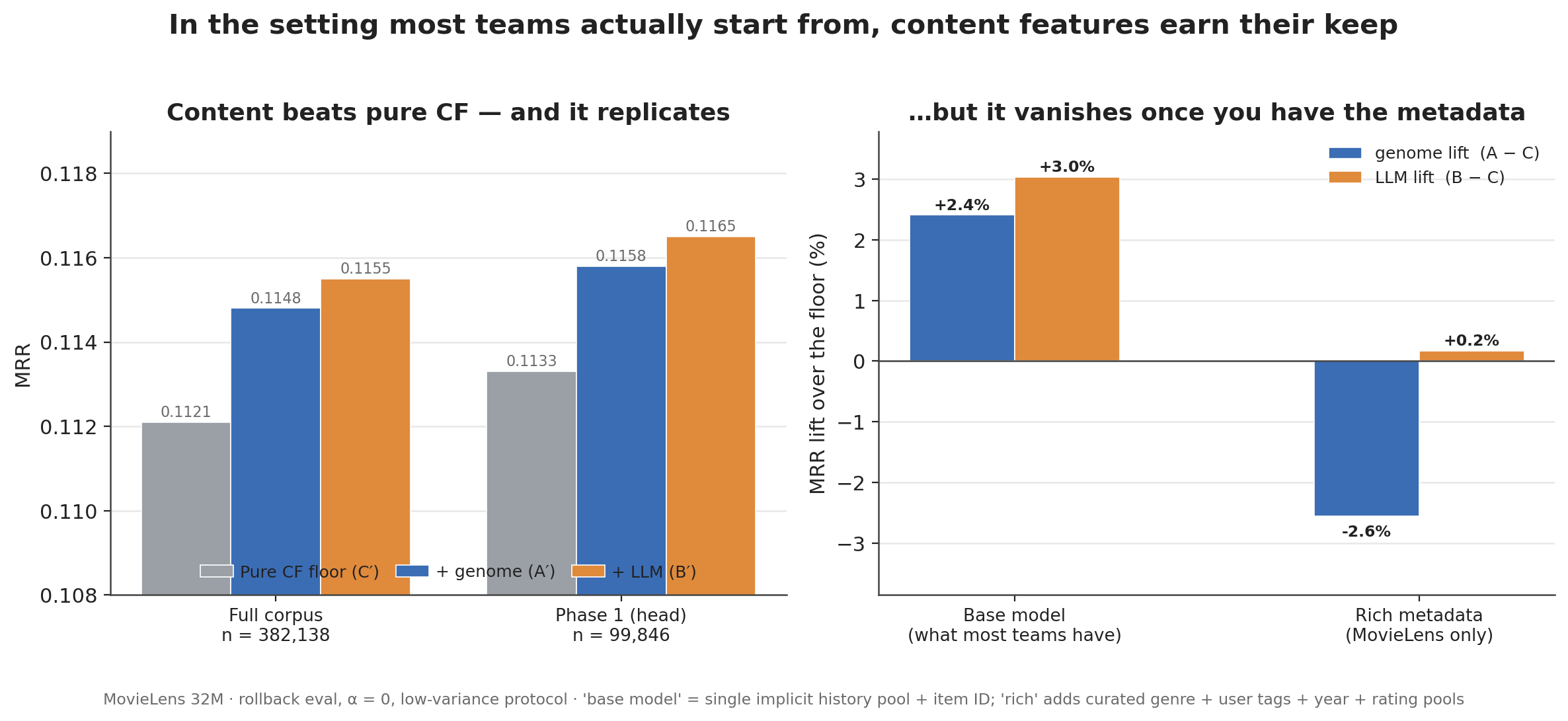
Figure 1. Left: in the base (universal) model, content beats the pure-CF floor and the ordering C′ < A′ < B′ replicates across both corpora. Right: add the curated genre + user tags + year + rating pools, and the same content slot’s lift over the floor collapses to ~0 / negative — genome and LLM go redundant with the cheap metadata (§6).
Three takeaways:
-
Content clears the floor — both sources do. Against a genuine pure-CF baseline, genome adds +2.4% MRR (A′−C′ = +0.0027) and the LLM +3.0% (B′−C′ = +0.0034). When the model has nothing else to lean on, a content vector earns real lift. That’s the question the metadata-rich setup (§6) couldn’t even ask.
-
The LLM matches the genome and noses ahead. B′ beats A′ on every metric and on every popularity tier (whole +0.0007, head +0.0007, and ≥0 across Q1–Q4). The margin is small — +0.6% MRR, within single-run noise on any one tier — but it’s consistent. The cheap, day-one option isn’t paying a quality tax against fifteen years of curated community data. If anything, it’s slightly ahead.
-
It replicates on a separate corpus. On the 4,461-movie Phase 1 head (n = 99,846), the same ordering holds: C′ 0.1133 < A′ 0.1158 < B′ 0.1165 (genome +2.2%, LLM +2.8% over floor). Each arm is still a single training seed. But a result that shows up across two corpora is firmer than two more seeds on one.
One caveat, to keep things honest: the measurable lift lives on the popular head (Q4/Q3), not the deep tail. Down at MovieLens’s ≥200-rating floor, every arm is near-zero and there are too few examples to tell them apart. The real cold-start regime — where content should matter most — can’t be benchmarked against the genome at all (§8).
5. Why it works — what each source actually knows
Both spaces sit on the same axes, so we can correlate them head-on: for each of the 132 LLM dims, compute the Pearson r against its mapped genome tag(s) across all 9,375 movies.
What’s “Pearson r”? One number from −1 to +1 for how tightly two sets of scores move together. Take one axis — say western — and line up the genome score and the LLM score across all 9,375 movies. r ≈ 1 means whenever genome calls a movie western, so does the LLM, movie for movie. r ≈ 0 means the two are unrelated — knowing one tells you nothing about the other. r ≈ −1 means they move in opposite directions. So high r = the LLM and genome agree.
Mean r = 0.598, median 0.608; 99 of 132 dims at r ≥ 0.5, none below 0.1. The two are measuring the same thing. By group: visual 0.70, setting 0.68, and provenance 0.64 agree highest; themes and tone sit at 0.56; reception is lowest at 0.42.
- Best axes (factual): vampires 0.94, documentary 0.89, animated/anime 0.88, western 0.86, WWII 0.86, time-travel 0.85.
- Worst axes (crowd-sentiment): imdb_top_250 0.16, criterion 0.18, palme_dor 0.27.
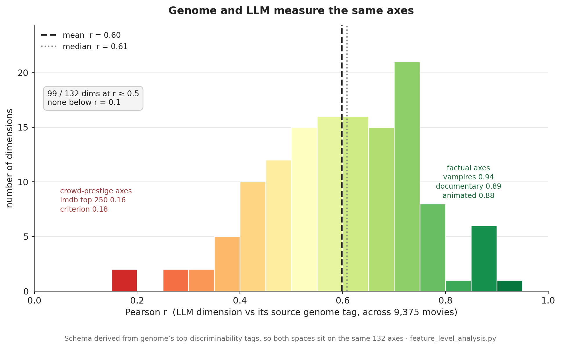
Figure 2. Per-dimension agreement between each LLM feature and its source genome tag, across all 9,375 movies (mean r = 0.60; 99 of 132 dims at r ≥ 0.5, none below 0.1). Agreement is highest on factual axes — genre, era, medium — and lowest on crowd-prestige axes (imdb top 250, criterion): exactly the slice an LLM can’t read from a synopsis.
That split is the mechanism. The LLM reproduces nearly all of genome’s signal on the axes it can read from text — genre, setting, provenance, factual medium. That’s why B′ matches A′ on the bulk metrics. The two only really diverge on the low-agreement axes, and it cuts both ways:
- Only genome holds: crowd-prestige (“masterpiece,” “imdb top 250”), fine niche sub-genre detail (The Good, the Bad and the Ugly — genome’s “spaghetti western” + “ennio morricone” against the LLM’s coarser “western”), and subjective aesthetics.
- Only the LLM adds: clean plot facts genome buries — “artificial_intelligence” for 2001, “based_on_book” for Die Hard, “hitman”/“conspiracy” for Sicario.
And here’s the key part. Genome’s exclusive axes are mostly crowd-sentiment and prestige, which track popularity more than content — so they don’t buy a ranking advantage. In the base model the LLM’s plot-facts slightly outweigh them.
Qualitative color (seed-dependent — not a headline). Canary top-10s give the two sources different personalities. Genome leans niche-canon-pure. The LLM leans era and modern-subgenre, but drifts to blockbusters on niche genres. Five disagreements:
| Persona | Genome (A) leans | LLM (B) leans |
|---|---|---|
| Sci-Fi | cerebral — Brazil, Gattaca, Forbidden Planet | popcorn — Fifth Element, T2, Total Recall |
| Crime | drifts to finance — Big Short, Margin Call | nails gritty — Sicario 2, Hell or High Water |
| Western | tight canon — Searchers, Rio Bravo | drifts to war epics — Patton, Braveheart |
| Arthouse | slow-burn — Stalker, In the Mood for Love | prestige — Fight Club, American Beauty |
| Horror | 90s slashers — Scream 2/3, Ring | 2000s gore — Saw II/IV/V, House of Wax |
Treat this strictly as color. The quantitative metrics carry the conclusion, not the canary.
6. Does the curated metadata change the answer? (the follow-up)
Here’s the obvious objection to §4: “you crippled the model — what about a feature-rich one?” Fair. So I re-ran all three arms in the rich model, with genome’s curated genre, 306 user tags, year, and the rating-derived pools added back.
The content lift collapses for both sources. On the same protocol the floor even edges out the genome:
| Whole-corpus MRR | C — no content | A — genome | B — LLM |
|---|---|---|---|
| Rich model | 0.1174 | 0.1144 | 0.1176 |
| Base model (§4) | 0.1121 | 0.1148 | 0.1155 |
Genome landing below the floor (A−C = −0.0030) doesn’t mean “content is useless.” Arm C still has genre, tags, and year, so genome is just a second copy of what’s already in there. The real tell is what each arm loses when you strip that metadata out:
| Arm | rich → base (whole-corpus MRR) | Δ |
|---|---|---|
| Floor (C → C′) | 0.1174 → 0.1121 | −0.0053 |
| LLM (B → B′) | 0.1176 → 0.1155 | −0.0021 |
| Genome (A → A′) | 0.1144 → 0.1148 | +0.0004 |
This substitution ladder (it replicates on Phase 1) is the whole result. Genome loses nothing when you drop genre and tags — it just rebuilds them, because genome tags basically are that metadata in another form. The LLM loses a little: its plot/tone/theme/cast basis is partly orthogonal, so it only partly backfills. The floor loses the most. That genome > LLM > none ranking is direct evidence the LLM features overlap less with cheap metadata — meaning they carry more genuinely additive signal.
Net: with a rich metadata stack, an extra content vector is redundant. Without one — which is most teams — it’s a real +2–3% lift, and the LLM is the less redundant of the two. The true lift for a given team lands somewhere in that bracket, closer to the base end the less curated metadata they own.
7. The payoff: feasibility, speed, cost
This is where “good enough” cashes out. The point was never that the LLM features are 1% better. It’s that they’re the option a real team can actually build. Dimension by dimension (every replication dollar figure below is a labeled estimate — the genome papers publish none):
| Dimension | Genome (GroupLens) | LLM extraction (this repo) |
|---|---|---|
| Human labeling | 50,203 judgments (676 volunteers); ~$5k–23k (central ~$10k) to buy as crowd labor today (est) | Zero |
| Binding prerequisite | ~15 years of community tagging (186k users / 17M ratings / 246k tag applications, since 1997) + crawled IMDb reviews — accrues with usage, not buyable quickly | The item’s own text — exists day one |
| Specialist engineering | LSI/SVD features + rating-affinity + text-mining + a 6-model regression bake-off; weeks–months (est) | Scraper + schema derivation + 6 grouped prompts; a few engineer-days |
| Direct $ (this corpus) | ~$10k survey + tens of $k labor, only if you already own that tagging history; ~$85–210k to hand-curate without it (est) | ~$0 marginal as run; ~$170–220 if reproduced on the metered API (Sonnet $3/$15) |
| Wall-clock to build, full corpus | Accreted over ~15 years of community use | ~1 day for all ~9,375 items — independent calls, fanned out in parallel |
| Time-to-first-vector, new item | Effectively never until the crowd tags it | Sub-hour, zero-shot from text |
| Maintenance / new domain | Re-survey + re-crawl + re-train; new domain = redo everything | Parallel API calls per item |
| Quality (universal setting) | A′: MRR 0.1148 | B′: 0.1155 — matches, edges ahead, +2–3% over the floor |
Three legs:
- Feasibility / build-vs-build. The genome needs a mature tagging history plus specialist research. The LLM needs item text. The LLM side is cheap but not “$0” — full-corpus extraction ran in a single day and ate ~84% of one week’s Sonnet quota on a Claude Max plan (≈$0 marginal under the subscription; ~$170–220 if you reproduce it on the metered API). Direct-dollar savings run roughly 1–3 orders of magnitude. But the claim that holds up is feasibility, not price: for a company without that tagging history, the genome path isn’t expensive — it’s unavailable.
- Speed / cold-start. Time-to-first-content-vector for a brand-new item: under an hour (scrape + six calls) against the genome’s effectively never — its input features are all zero until the crowd tags the item.
- Cold-start bootstrapping (enabled, not measured here). A sub-hour content vector lets you compute content-space nearest neighbors and drop a new item into the traffic of users who already get its most-similar items — warming up its collaborative embedding on far fewer impressions (cf. DropoutNet, NeurIPS 2017). I didn’t build or measure that here. But the experiment backs the premise it rests on: the r≈0.60 agreement and the Toy Story / Godfather similarity checks show the content NN is meaningful. Mind the axis, though. NN-seeding is a rich-content-vs-no-content win, so genome enables it too. It’s LLM-specific only at true cold start, where genome doesn’t exist to NN on in the first place.
“Neural ≠ cheaper” sidebar. The 2021 genome refresh (TagDL, a PyTorch MLP) bought ~2.6% MAE and changed none of the data prerequisites — same survey, same tagging history. And the genome team’s own 2026 cross-domain paper ran straight into the prerequisite wall extending to Amazon — “the absence of … item-tag ratings and tag applications” — had to reuse old survey labels, and took a measured accuracy hit. The strongest evidence that the prerequisite is binding comes from the people who built the genome.
8. Limitations
Limitations, stated plainly:
- Single seed per arm — but cross-corpus replicated. No seed ensembles, no CIs. But the ordering (C′ < A′ < B′, B′ edging A′) and the substitution ladder both replicate across the full and Phase 1 corpora — firmer than extra seeds on one. Read per-tier A′-vs-B′ gaps ≤ 0.0007 MRR as “matches,” carried by direction, not magnitude.
- The “universal” floor isn’t perfectly implicit. The base model’s history pool is un-rated, so truly implicit. But the content arms’ user-side pooling still rating-weights each item’s content vector. A strictly implicit deployment would weight uniformly. The effect is small — just how content gets averaged over history — but it’s a real residual behind the “no ratings” claim.
- Two separate filterings, easy to mix up — and we filtered neither genome one. (1) Our corpus: all arms train and eval on the 9,375 movies with >200 ratings — our cutoff on MovieLens 32M’s 87,585 titles. Both sources cover it fully (genome scores all 9,375), so the fight is scale-matched. (2) The genome’s own ceiling: GroupLens only ever published genome for 16,376 movies (~19% of the catalog). The other ~81% are too sparsely tagged for their model. So our eval can’t see the gap that matters most: across that ~81% the genome simply doesn’t exist, while the LLM scores any title from its text (~$1.6–2k metered for the whole catalog, est). The numbers almost certainly understate the feasibility gap.
- A true cold-start head-to-head is structurally impossible. Cold start is where an LLM vector should pay off (§7), but you can’t benchmark it against the genome — the genome isn’t there. And the lift we do measure lives on the popular head. At the ≥200-rating floor every arm is near-zero on the deep tail, so the real cold-start regime goes unmeasured (and has no genome arm to compare against anyway).
- Single LLM. Claude Sonnet only, no cheaper-model bake-off. So this supports “Sonnet-class extraction matches genome,” not “any cheap model would.”
- The shared taxonomy is genome’s — by design, to handicap the LLM (§2), not because the method needs one. We held the LLM to genome’s tags so the match is tag-for-tag on its home turf. What’s left open: we showed an LLM can fill a curated taxonomy to genome quality. An LLM drafting a richer one — which the scrape data would support — is argued in §2, not benchmarked.
- Movies are a text-rich, easy case. Every item ships with a Wikipedia plot, TMDB cast, and reviews. The extractor never had to work from thin text. Whether it still tracks a gold-standard signal on items with three sentences of description is unmeasured.
- Cost is amortized, not zero. The ~$0 is marginal dollars under a flat-rate subscription, not a per-call API figure.
- Crowd-sentiment is a scope choice, not a hard limit. Genome’s pure-sentiment tags (“masterpiece,” “overrated”) are where the LLM trails (r≈0.16–0.18) — not because an LLM can’t read sentiment, but because we only scraped Wikipedia and TMDB. Point the same pipeline at reviews and it recovers it.
- Prestige-as-popularity leakage. Scraped box-office and IMDb-rating in the reception group are quasi-popularity signals, which works against isolating content. That’s why that group is separately ablatable.
- Possible training-data contamination — and it cuts toward the LLM. MovieLens gets discussed online a lot and the genome tags are public, so the extractor might be partly reciting genome knowledge instead of reading the synopsis. That would inflate the r≈0.60 agreement on this corpus specifically. A fresh-catalog replication is the clean check.
9. Takeaway
No pre-existing tagging history? Scrape the text. For the recommender most teams are actually building — implicit interactions, item text, none of MovieLens’s curated metadata — LLM-extracted content features are the pragmatic default. They earn a real lift over collaborative filtering alone, on the gold-standard genome’s own axes, matching it and edging it by a small but consistent margin. (Already own a rich curated-metadata stack? Then an extra content vector is redundant either way, and the genome’s fifteen-year provenance buys you nothing you couldn’t scrape in a day.)
The deeper point: genome and LLM are two generations of the same idea. Both turn cheap signals into a dense content matrix. GroupLens did it with a 50,000-judgment survey and regression, standing on fifteen years of community data. The LLM does it from the item’s own text — and drops the community, the tag-data dependence, and the cold-start wall in one move. It gives up a thin slice of crowd-curated nuance to run on day one, for any item, at any company. Fifteen years of provenance, or a day of scraping, for the same axes. For the content-feature problem most teams actually have, that’s the trade you want.
Appendix — Sources & notes
Results come from a held-out rollback evaluation under a low-variance protocol (seeded, 160k steps) — full corpus all 19,134 validation users / 382,138 ranking examples, replicated on a 4,461-movie head corpus. Genome-construction facts come from GroupLens’s tag-genome work (Vig, Sen & Riedl, 2010/2012) and its later cost/feasibility line (TagDL, SIGIR ‘21; book genome, CHIIR ‘22; cross-domain genome, CHIIR ‘26), with cost anchors from public MTurk/Prolific and Pandora figures. Every dollar figure is a labeled estimate — the genome papers publish none. Full code, data pipeline, and per-tier eval outputs are in the repository.